Category Archives: Mathematical Art

Estimating The Fractal Dimension of the Spiders of Mars

Spider Terrain (NASA/JPL/UArizona )

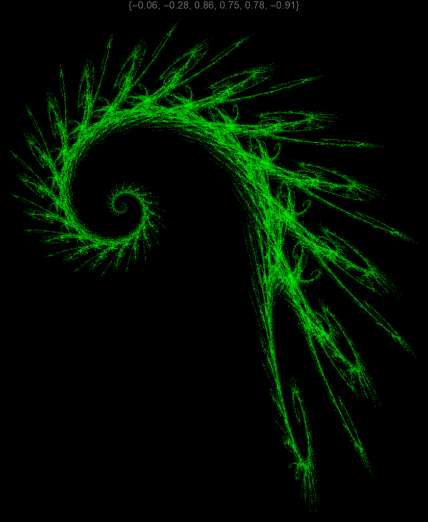
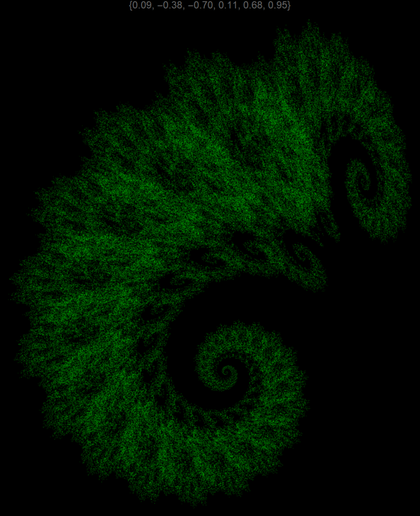
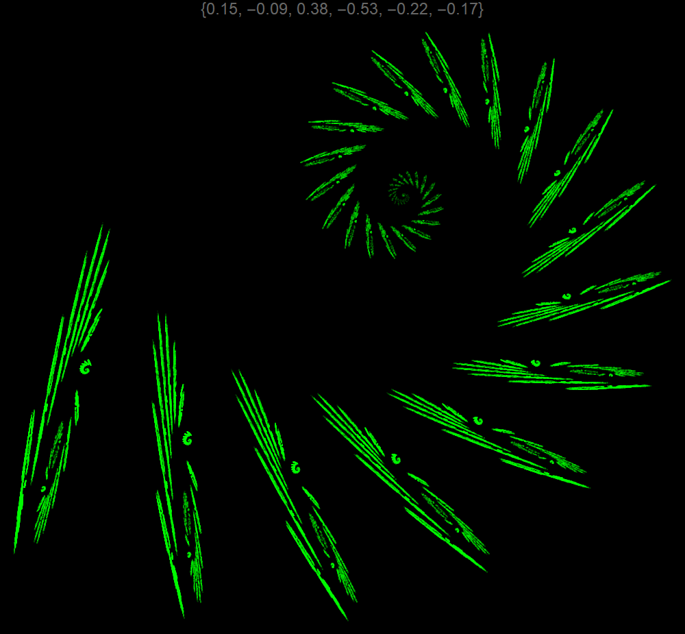
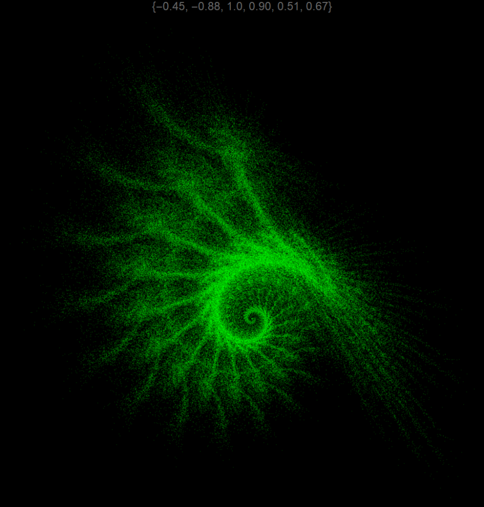
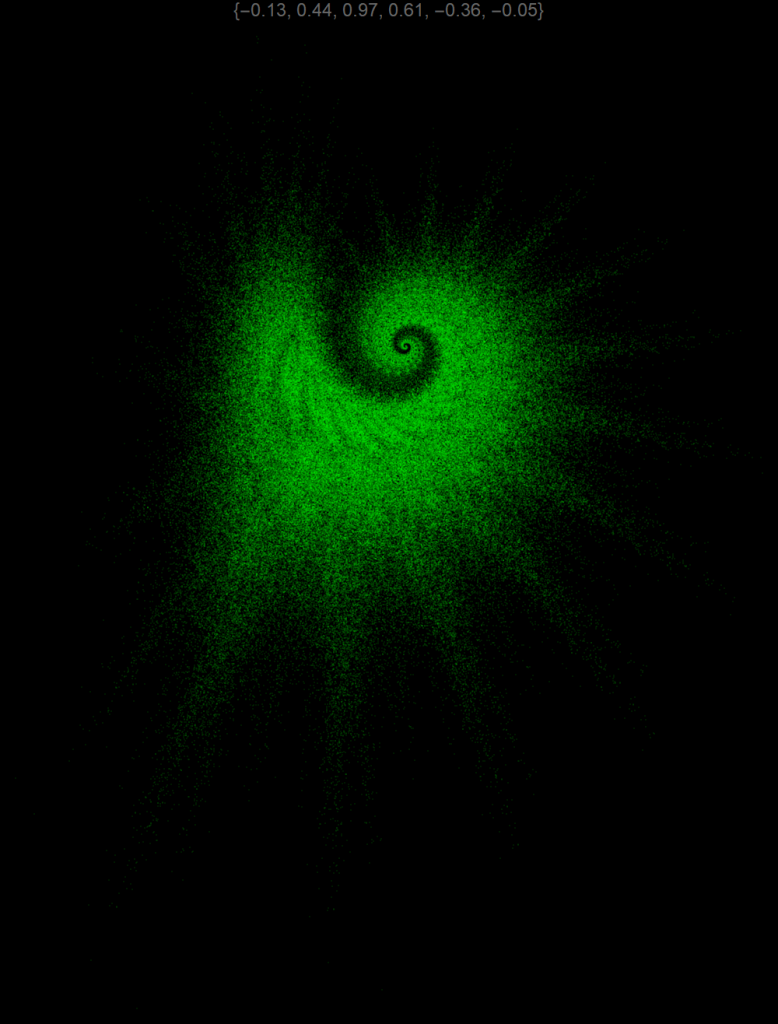
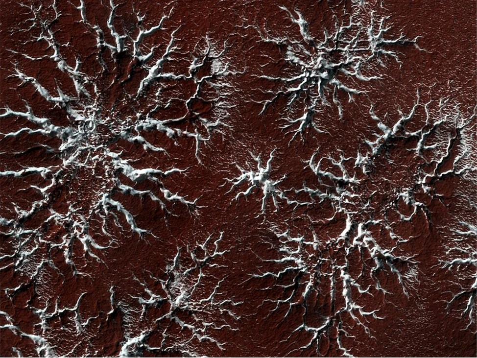
Above is an image of “dry ice spiders” on Mars. Every spring the Sun warms up the Martian south polar icecap and causes jets of carbon-dioxide gas to erupt through the icecap. These jets carrying dark sand into the air and spraying it for hundreds of feet around each jet forming these wonderful spider-like structures. Notice how they look very much like fractals.

Just for fun, and because I had a week off, I wondered if I could calculate, or really estimate the fractal dimension of these structures. To do this, I decided to use the box-counting dimension, which gives a bound on the fractal dimension. Rather than give a careful description here I will point to the following link.

I did this in a few stages using Mathematica. First I needed to get a form of the image that can be used.

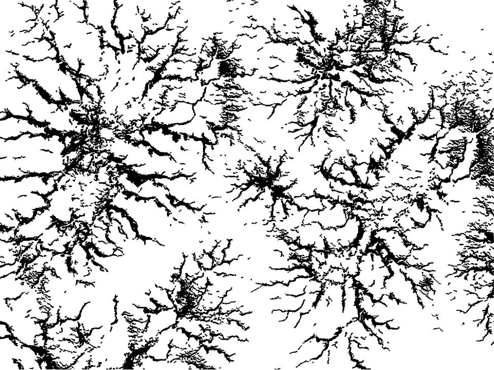
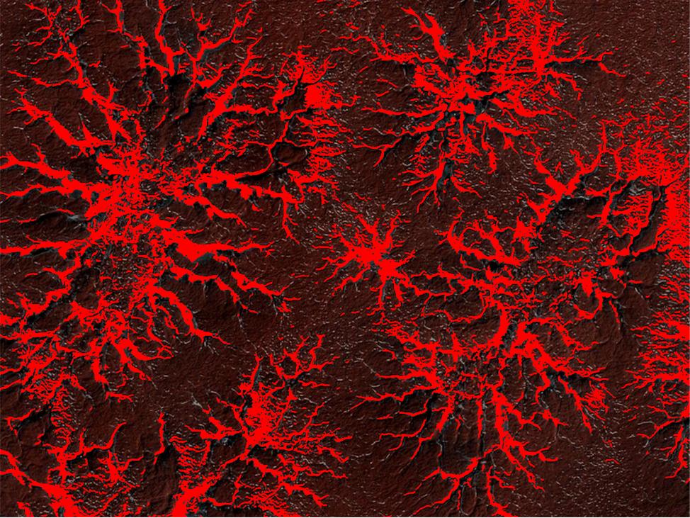
The image of the left is what I then used as the fractal that I wanted to estimate the box-counting dimension of. The image of the right is the overlay of the original image and the “extracted” image. This shows that it is not perfect, but it will do for now.

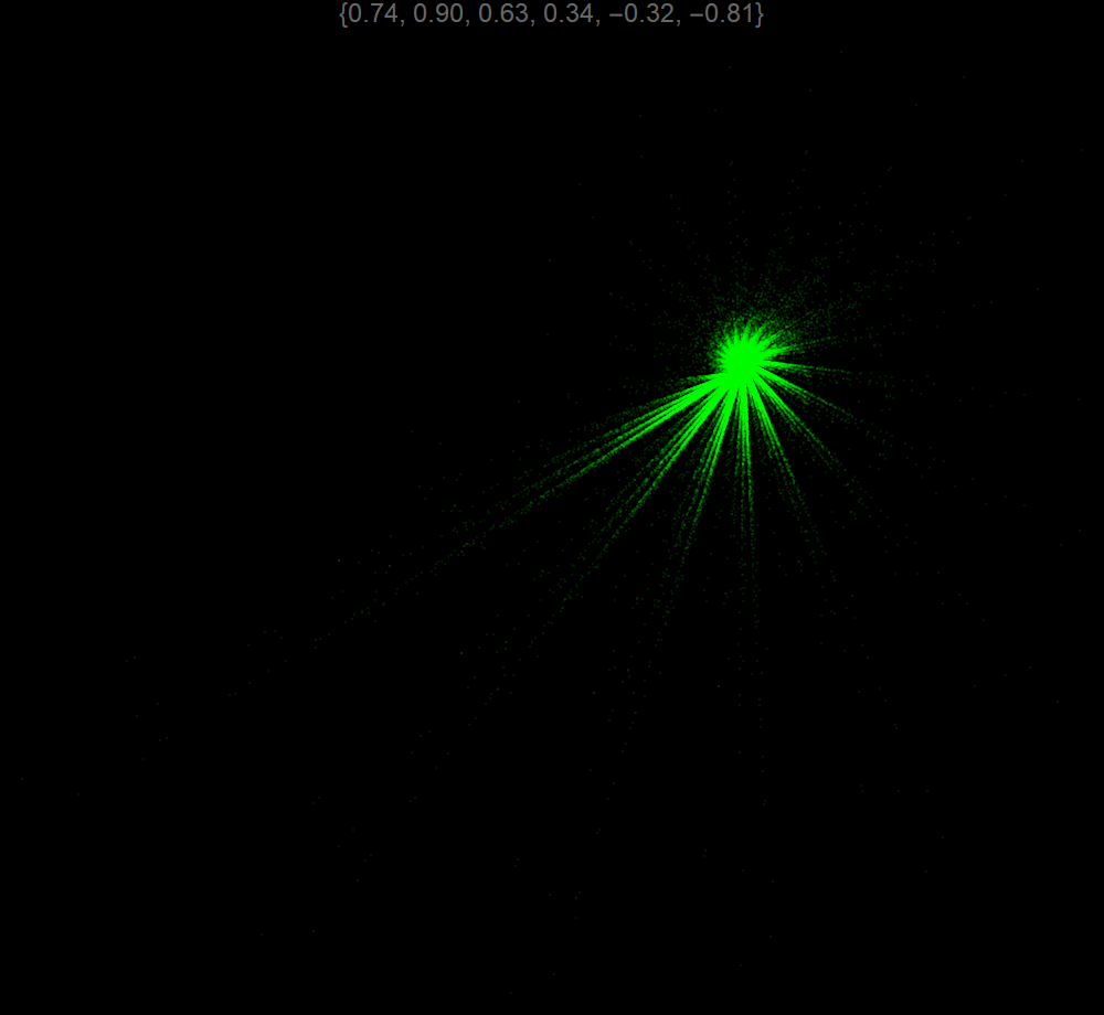
Then I needed to write a Mathematica notebook that will give an estimate of the box-counting dimension. Of course, before I applied it to the spider question, I tested it on fractals with know fractal dimensions. It worked very well in general. Thus, I am confident that the estimate for the spider landscape is reasonable (modulo details of how I created the simpler black and white image).

So, what do I get for the box-counting dimension?

dimbox= 1.758 ± 0.013

Before anyone takes that figure too seriously, one should study many more of these spiders and see what range of values ones gets. Also the sensitivity to how I have “extracted” the fractal from the original should be tested. I have no idea if this has been done before or if it is interesting to anyone, like i said just for fun.

More fun with IFS Fractals

I have been playing with some iterated function systems again. These images were built using two affine transformations, one being a rotation through 20 degree composed a scaling of 90% and the second is a general affine transformation chosen at random.

Some of the best of these results I have attached here. I have added colors for ascetic reasons. Enjoy.

Below are some of the results of the random search. Some are more interesting than others.

An IFS fractal

IFS

Another IFS pseudo-fractal image. I am now experimenting with how to colour them. Here have an opacity that encodes the number of times a point is visited, but also as a dynamical system the points are ordered. So I have added a colour based on the order at which the points are visited.

On a variant of rhodonea curves

Rhodonea curves or rose curves are plots of a polar equation of the form
\(r = \cos(k \theta)\).

If we specialise to equations with

\(k= \frac{n}{d}\)

for n and d integers (>0), then we have plots of the form below. In the table n runs across and d down

Now, just for fun I considered a slight variant of this given by

\(r = \cos( k \theta) – k\)

The plots are as follows

For another variant I considered

\(r = \cos( k \theta) – k^{-1}\)

I am not sure there is anything mathematically deep here, I just like the images and classify this as some basic mathematical art.

More experiments with random walks

I have again been playing with some random walks, using the same method as here. This time I used 1000000 iterations and added some colour.

Below are random walks, on the plane (not a lattice) for which step size gets (on average) smaller and smaller with each step. I pick the step size using the Maxwell-Boltzman distribution (with a =1) and a suitable scaling which depends on the iteration parameter. I the add a opacity depending on how many times the points are visited: bright white means a lot, while grey means not many and black never.

walk

walk

walk

walk

Once again, these images are rather for artistic purposes than scientific purposes.

This is like so random…

Below are random walks on the plane (not a lattice) for which step size gets (on average) smaller and smaller with each step. I pick the step size using the Maxwell-Boltzman distribution (with a =1) and a suitable scaling which depends on the iteration parameter. I the add a opacity depending on how many times the points are visited: bright white means a lot, while grey means not many and black never.

I may play with these further, but they make some interesting pattens. We have approximate self-similarity and so these patterns have fractal-like properties. Anyway, enjoy….

random10

random1

random2

random5

These images were created for artistic rather than scientific reasons. That said, random walks are have been applied to many fields including ecology, economics, psychology, computer science, physics, chemistry, and biology.

Probably the most famous application of a random walk is to Brownian motion, which describes the trajectory of a tiny particle diffusing in a fluid. I have no idea if there is anything scientific in these images, but I would not be surprised if for small step sizes we have approximately Brownian motion. However, I would need to think a lot more about this before making concrete statements.