Renaming the Higgs boson

Higgs

Peter Higgs was treated as something of a rock star and the rest of us were barely recognised. It was clear that Higgs was the dominant name because his name has become associated with the boson.

Prof Carl Hagen Rochester University, New York (BBC World News)

As you are all probably aware, on the 14th of March 2013 the ATLAS and CMS collaborations at CERN’s Large Hadron Collider (LHC) presented new results that further support the discovery of the so called Higgs boson [1].

This has all reignited the debate on the naming of the standard model scalar boson, as “Higgs” only reflects one of the physicists who made early contributions to the generation of mass within the standard model.

In 1964 Robert Brout & François Englert [2], Peter Higgs [4] and Gerald Guralnik , Carl Hagen & Tom Kibble [4] published papers proposing similar, but different mechanisms to give mass to particles in gauge theories, such as the standard model. All of the six physicists were awarded the 2010 J. J. Sakurai Prize for Theoretical Particle Physics for their work on spontaneous symmetry breaking and mass generation.

winners
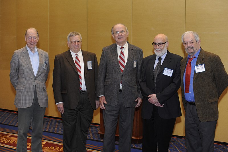
2010 Sakurai Prize Winners – (L to R) Kibble, Guralnik, Hagen, Englert, and Brout

The trouble now is that the nomenclature Higgs boson has been around for a while now and remaining it could probably course unnecessary confusion. Also, it is not clear who should decide the new name. Nomenclature in physics, and indeed mathematics, arises largely due to popular usage. The initial name may come from the discoverer, but it still takes the community to use this nomenclature before it becomes standard. Thus, the community would have to change nomenclature and this cannot really be imposed from “outside”.

Naming the particle after the six physicists as BEHGHK-boson, which would be pronounced “berk-boson” is one one possible solution, but not a very nice one!

Pallab Ghosh (Science correspondent, BBC News) discusses this further here.

References
[1] New results indicate that particle discovered at CERN is a Higgs boson, CERN press office 14th March 2013.

[2] Englert, F.; Brout, R. (1964). “Broken Symmetry and the Mass of Gauge Vector Mesons”. Physical Review Letters 13 (9): 321.

[3] Higgs, P. (1964). “Broken Symmetries and the Masses of Gauge Bosons”. Physical Review Letters 13 (16): 508.

[4]Guralnik, G.; Hagen, C.; Kibble, T. (1964). “Global Conservation Laws and Massless Particles”. Physical Review Letters 13 (20): 585.

Compatible homological vector fields

In an earlier post, here, I showed that the homological condition on an odd vector field \(Q \in Vect(M)\), on a supermanifold \(M\), that is \(2Q^{2}= [Q,Q]=0\), is precisely the condition that \(\gamma^{*}x^{A} = x^{A}(\tau)\), where \(\gamma \in \underline{Map}(\mathbb{R}^{0|1}, M)\), be an integral curve of \(Q\).

A very natural question to answer is what is the geometric interpretation of a pair of mutually commuting homological vector fields?

Suppose we have two odd vector fields \(Q_{1}\) and \(Q_{2}\) on a supermanifold \(M\). Then we insist that any linear combination of the two also be a homological vector field, say \(Q = a Q_{1} + b Q_{2}\), where \(a,b \in \mathbb{R}\). It is easy to verify that this forces the conditions

\([Q_{1}, Q_{1}]= 0 \), $latex[Q_{2}, Q_{2}]= 0 $ and \([Q_{1}, Q_{2}]= 0 \).

That is, both our original odd vector fields must be homological and they mutually commute. Such a pair of homological vector fields are said to be compatible. So far this is all algebraic.

Applications of pairs, and indeed larger sets of compatible vector fields, include the description of n-fold Lie algebroids [1,3] and Q-algebroids [2].

The geometric interpretation
Based on the earlier discussion about integrability of odd flows, a pair of compatible homological vector fields should have something to do with an odd flow. We would like to interpret the compatibility of a pair of homological vector fields as the integrability of the flow of \(\tau = \tau_{1} + \tau_{2}\). Indeed this is the case;

Consider \(\gamma^{*}_{\tau_{1} + \tau_{2}}(x^{A}) = x^{A}(\tau_{1} + \tau_{2}) = x^{A}(\tau_{1}, \tau_{2})\), remembering that we define the flow via a Taylor expansion in the “odd time”. Expanding this out we get

\( x^{A}(\tau_{1}, \tau_{2}) = x^{A} + \tau_{1}\psi_{1}^{A} + \tau_{2}\psi_{2}^{A} + \tau_{1} \tau_{2}X^{A}\).

Now we examine the flow equations with respect to each “odd time”. We do not assume any conditions on the odd vector fields \(Q_{1}\) and \(Q_{2}\) at this stage.

\(\frac{\partial x^{A}}{\partial \tau_{1}} = \psi_{1}^{A} + \tau_{2}X^{A} = Q_{1}^{A}(x(\tau_{1}, \tau_{2}))\)
\(= Q_{1}^{A}(x) + \tau_{1}\psi^{B}_{1} \frac{\partial Q^{A}_{1}(x)}{\partial x^{B}} + \tau_{2}\psi^{B}_{2} \frac{\partial Q^{A}_{1}(x)}{\partial x^{B}} + \tau_{1}\tau_{2}X^{B} \frac{\partial Q^{A}_{1}(x)}{\partial x^{B}}\),

and
\(\frac{\partial x^{A}}{\partial \tau_{2}} = \psi_{2}^{A} {-} \tau_{1}X^{A} = Q_{2}^{A}(x(\tau_{1}, \tau_{2}))\)
\(= Q_{2}^{A}(x) + \tau_{1}\psi^{B}_{1} \frac{\partial Q^{A}_{2}(x)}{\partial x^{B}} + \tau_{2}\psi^{B}_{2} \frac{\partial Q^{A}_{2}(x)}{\partial x^{B}} + \tau_{1}\tau_{2}X^{B} \frac{\partial Q^{A}_{2}(x)}{\partial x^{B}}\).

Then equating coefficients in order of \(\tau_{1}\) and \(\tau_{2}\) we arrive at three types of equations

i) \(\psi_{1}^{A} = Q_{1}^{A}\), \(\psi^{B}_{1} \frac{\partial Q_{1}^{A}}{\partial x^{B}}=0\) and \(\psi_{2}^{A} = Q_{2}^{A}\), \(\psi^{B}_{2} \frac{\partial Q_{2}^{A}}{\partial x^{B}}=0\).

ii) \(X^{A} = \psi^{B}_{2} \frac{\partial Q_{1}^{A}}{\partial x^{B}}\) and \(X^{A} = {-}\psi^{B}_{1} \frac{\partial Q_{2}^{A}}{\partial x^{B}}\).

iii) \(X^{B} \frac{\partial Q_{1}^{A}}{\partial x^{B}} =0\) and \(X^{B} \frac{\partial Q_{2}^{A}}{\partial x^{B}} =0\).

It is now easy to see that;

i) implies that \([Q_{1}, Q_{1}] =0 \) and \([Q_{2}, Q_{2}] =0 \) meaning we have a pair of homological vector fields.

ii) implies that \([Q_{1}, Q_{2}]=0\), that is they are mutually commuting, or in other words compatible.

iii) is rather redundant and follows from the first two conditions.

Thus our geometric interpretation was right.

References
[1] Janusz Grabowski and Mikolaj Rotkiewicz, Higher vector bundles and multi-graded symplectic manifolds, J. Geom. Phys. 59(2009), 1285-1305.

[2]Rajan Amit Mehta, Q-algebroids and their cohomology, Journal of Symplectic Geometry 7 (2009), no. 3, 263-293.

[3] Theodore Th. Voronov, Q-Manifolds and Mackenzie Theory, Commun. Math. Phys. 2012; 315:279-310.